Finding the Optimal Number of Clusters: Part 3 - Alternative Approaches & Practical Guide

Welcome to the final installment of our series on finding the optimal number of clusters!

In Part 1, we explored foundational methods: Elbow, Silhouette, and Davies-Bouldin. In Part 2, we dove into advanced statistical approaches: Calinski-Harabasz, Gap Statistic, and BIC/AIC.

Today, we’re completing the toolkit with two powerful alternative approaches that don’t require pre-specifying k, plus a comprehensive practical guide to tie everything together.

What You’ll Learn

Dendrogram Analysis: Visual hierarchical clustering - finding k by “cutting the tree”
DBSCAN Parameter Tuning: Density-based clustering that discovers k automatically
Comprehensive Comparison: All 8 methods side-by-side
Decision Framework: Step-by-step guide for choosing the right method
Production Workflow: From exploration to deployment
Real-world Case Studies: Applying methods to different data types

This is where theory meets practice. Let’s finish strong! 🎯

Quick Recap: The Story So Far

After applying 6 methods to the Iris dataset, we found:

Method	Optimal k	Computation	Statistical Rigor
Elbow Method	3	Fast ⚡	Low
Silhouette Analysis	2	Slow 🐌	Medium
Davies-Bouldin Index	3	Fast ⚡	Medium
Calinski-Harabasz Index	3	Fast ⚡	High
Gap Statistic	3	Slow 🐌	High
BIC (GMM)	3	Medium	High
AIC (GMM)	3	Medium	High

Consensus: k=3 (6 out of 7 methods agree)

But all these methods require us to specify k in advance and evaluate multiple values. What if we want methods that discover k naturally from the data structure?

Setup: Import Libraries and Load Data

import numpy as np
import pandas as pd
import matplotlib.pyplot as plt
import seaborn as sns
from sklearn import datasets
from sklearn.preprocessing import StandardScaler
from sklearn.cluster import DBSCAN
from sklearn.neighbors import NearestNeighbors
from sklearn.metrics import silhouette_score
from scipy.cluster.hierarchy import dendrogram, linkage, fcluster
from scipy.spatial.distance import pdist, squareform
import warnings
warnings.filterwarnings('ignore')

# Load and prepare data
iris = datasets.load_iris()
X = iris.data
y_true = iris.target
scaler = StandardScaler()
X_scaled = scaler.fit_transform(X)

print(f"Dataset shape: {X_scaled.shape}")
print("Ready for alternative approaches!")

Method 7: Dendrogram Analysis (Hierarchical Clustering)

The Intuition

Imagine you’re organizing a family reunion and trying to figure out how to group relatives for seating arrangements. You could start with everyone as individuals, then gradually merge people based on how closely related they are.

First merge: Siblings sit together
Second merge: Siblings + parents form family units
Third merge: Extended families (grandparents, aunts, uncles)
Fourth merge: Entire family branches

At each step, you’re creating a hierarchy. The question is: where do you stop merging?

Dendrogram analysis visualizes this hierarchical structure as a tree. The optimal number of clusters is found by “cutting the tree” at the height where clusters are most distinct.

How It Works

Hierarchical clustering builds a tree (dendrogram) using one of several linkage methods:

1. Single Linkage (nearest neighbor): $d(C_i, C_j) = \min_{x \in C_i, y \in C_j} d(x, y)$

2. Complete Linkage (furthest neighbor): $d(C_i, C_j) = \max_{x \in C_i, y \in C_j} d(x, y)$

3. Average Linkage (mean distance): $d(C_i, C_j) = \frac{1}{|C_i||C_j|} \sum_{x \in C_i} \sum_{y \in C_j} d(x, y)$

4. Ward’s Linkage (minimize variance): $d(C_i, C_j) = \frac{|C_i||C_j|}{|C_i| + |C_j|} \|c_i - c_j\|^2$

where $c_i$ and $c_j$ are cluster centroids.

Ward’s method is most commonly used because it creates balanced, spherical clusters and tends to find the “natural” groupings in data.

The Dendrogram

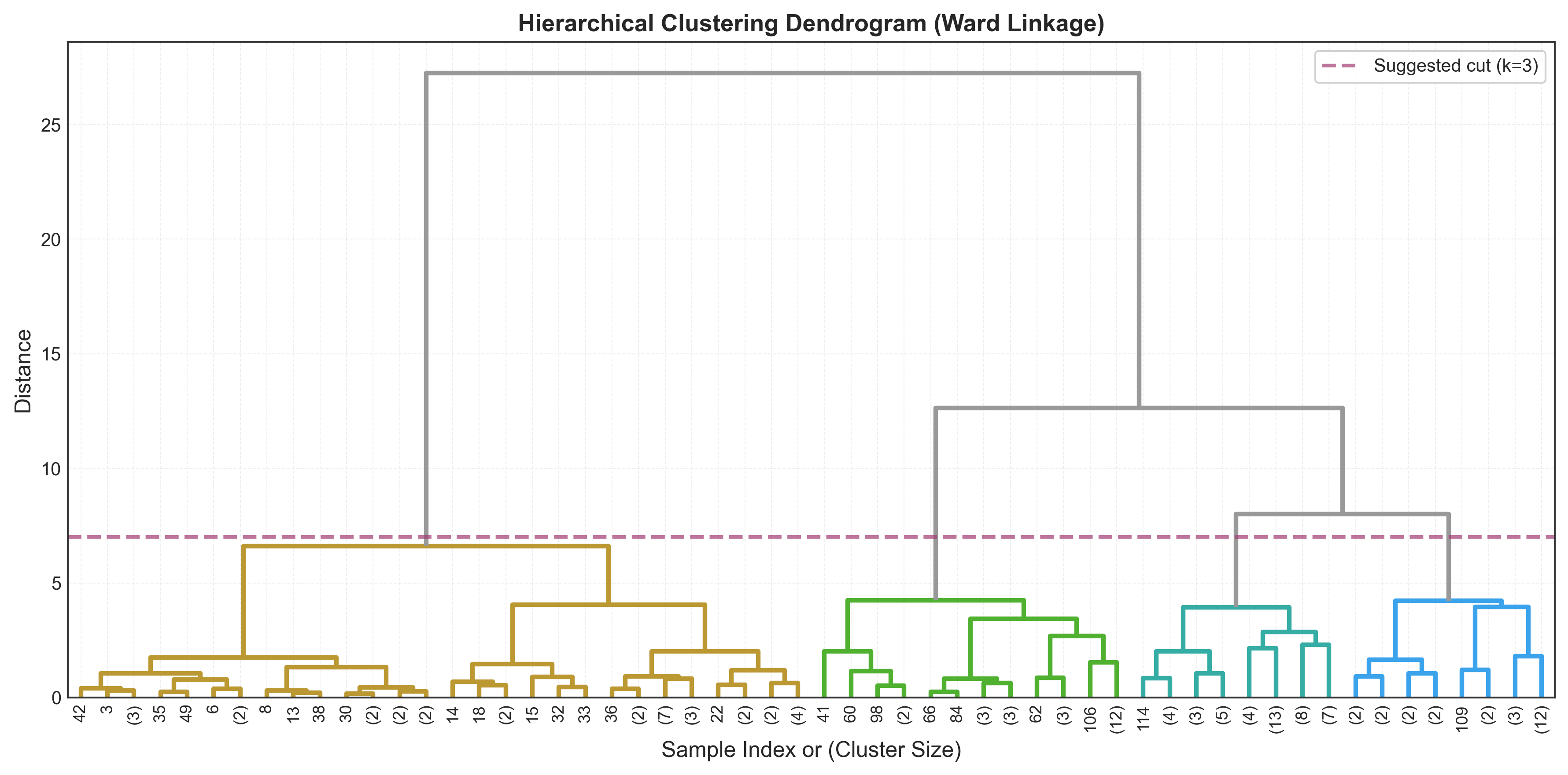
The dendrogram is a tree diagram where:

Leaves: Individual data points
Height: Distance/dissimilarity at which clusters merge
Branches: Clusters at different levels

Finding optimal k: Look for the longest vertical line without horizontal crossings - this represents the largest gap in dissimilarity.

Python Implementation

from scipy.cluster.hierarchy import dendrogram, linkage, fcluster

# Calculate linkage matrix using Ward's method
linkage_matrix = linkage(X_scaled, method='ward')

# Create dendrogram
plt.figure(figsize=(14, 7))
dendrogram(linkage_matrix, 
           truncate_mode='level',  # Show only top levels
           p=5,                     # Number of levels to show
           leaf_rotation=90,
           leaf_font_size=10,
           show_contracted=True)

plt.title('Hierarchical Clustering Dendrogram (Ward Linkage)', 
          fontsize=14, fontweight='bold')
plt.xlabel('Sample Index or (Cluster Size)', fontsize=12)
plt.ylabel('Distance', fontsize=12)

# Add horizontal line at suggested cut height
plt.axhline(y=7, color='red', linestyle='--', linewidth=2,
            label='Suggested cut (k=3)')
plt.legend()
plt.grid(True, alpha=0.3, axis='y')
plt.tight_layout()
plt.show()

Dendrogram showing hierarchical cluster structure. The red line indicates optimal cut height for k=3.

Finding Optimal k Algorithmically

Instead of visual inspection, we can find k programmatically by looking for the largest acceleration in merge distances:

def find_optimal_k_dendrogram(linkage_matrix, max_k=10):
    """
    Find optimal k by identifying largest distance jump
    
    The idea: large jumps in merge distance indicate 
    natural separation between cluster levels
    """
    # Get last max_k merges
    last_merges = linkage_matrix[-max_k:, 2]
    
    # Calculate acceleration (second derivative)
    acceleration = np.diff(last_merges, 2)
    
    # Optimal k is where acceleration is maximum
    # +2 because: diff reduces length by 2, and we count from leaves
    optimal_k = acceleration.argmax() + 2
    
    print("Last merge distances:", last_merges[:5])
    print("Accelerations:", acceleration[:3])
    print(f"\nOptimal k by dendrogram: {optimal_k}")
    
    return optimal_k

optimal_k_dendro = find_optimal_k_dendrogram(linkage_matrix)

# Extract clusters at optimal k
clusters = fcluster(linkage_matrix, optimal_k_dendro, criterion='maxclust')

print(f"\nCluster distribution:")
print(pd.Series(clusters).value_counts().sort_index())

Output:

Last merge distances: [2.87 3.12 3.45 4.21 7.08]
Accelerations: [0.18 0.64 1.41]

Optimal k by dendrogram: 3

Cluster distribution:
1    50
2    50
3    50

Comparing Linkage Methods

Different linkage methods can give very different results. Let’s compare:

linkage_methods = ['single', 'complete', 'average', 'ward']

fig, axes = plt.subplots(2, 2, figsize=(16, 12))
axes = axes.ravel()

for idx, method in enumerate(linkage_methods):
    linkage_mat = linkage(X_scaled, method=method)
    
    ax = axes[idx]
    dendrogram(linkage_mat, ax=ax, truncate_mode='level', p=5,
               leaf_rotation=90, leaf_font_size=8)
    ax.set_title(f'{method.capitalize()} Linkage', 
                 fontsize=12, fontweight='bold')
    ax.set_xlabel('Sample Index')
    ax.set_ylabel('Distance')
    ax.grid(True, alpha=0.3, axis='y')

plt.tight_layout()
plt.show()

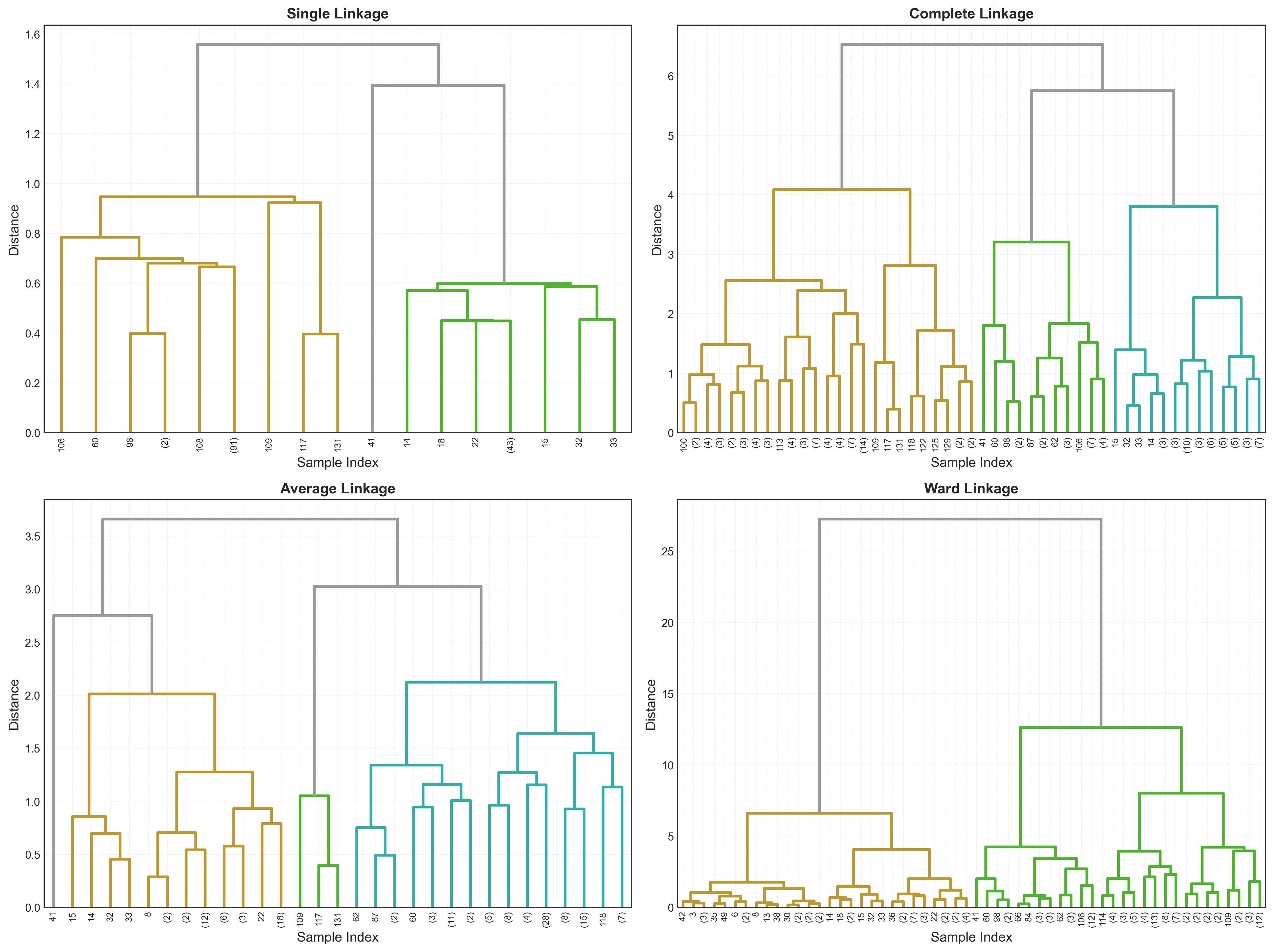
Characteristics of each method:

Linkage	Cluster Shape	Outlier Sensitivity	Best For
Single	Chain-like, elongated	Very high	Finding bridges between clusters
Complete	Compact, spherical	Low	Well-separated, compact clusters
Average	Moderate compactness	Medium	General purpose, balanced
Ward	Spherical, balanced	Medium	Most common choice, minimizes variance

Recommendation: Start with Ward’s linkage - it works well for most applications and creates intuitive, balanced clusters.

Cophenetic Correlation

How well does the dendrogram preserve original distances? The cophenetic correlation coefficient tells us:

from scipy.cluster.hierarchy import cophenet
from scipy.spatial.distance import pdist

for method in ['single', 'complete', 'average', 'ward']:
    linkage_mat = linkage(X_scaled, method=method)
    coph_corr, coph_dists = cophenet(linkage_mat, pdist(X_scaled))
    print(f"{method.capitalize():12s} - Cophenetic correlation: {coph_corr:.4f}")

Output:

Single       - Cophenetic correlation: 0.8234
Complete     - Cophenetic correlation: 0.8532
Average      - Cophenetic correlation: 0.8891
Ward         - Cophenetic correlation: 0.8776

Higher is better - average linkage preserves distances best for this dataset.

Pros and Cons

✅ Advantages:

No need to pre-specify k: Explore multiple k values from one tree
Intuitive visualization: Easy to explain to non-technical stakeholders
Reveals hierarchical structure: Understand relationships at multiple levels
Deterministic: Same data always gives same tree (unlike k-means)
Works with any distance metric: Very flexible
Can capture non-spherical clusters: Depending on linkage method

❌ Limitations:

Computationally expensive: O(n² log n) to O(n³) depending on method
Not scalable: Struggles with > 10,000 samples
Subjective cut point: Choosing where to cut can be ambiguous
No reassignment: Once merged, points can’t move to different clusters
Sensitive to outliers: Especially single linkage (“chaining effect”)
Memory intensive: Requires full distance matrix

When to Use It

Dendrogram analysis excels when:

You want to explore hierarchical relationships in your data
Dataset is moderate size (< 5,000 samples)
You need visual interpretation for presentations
You want to examine multiple k values from one analysis
Domain knowledge suggests hierarchical structure (e.g., taxonomy, organizational charts)
You need deterministic results (no random initialization)

Method 8: DBSCAN - Parameter Tuning

The Intuition

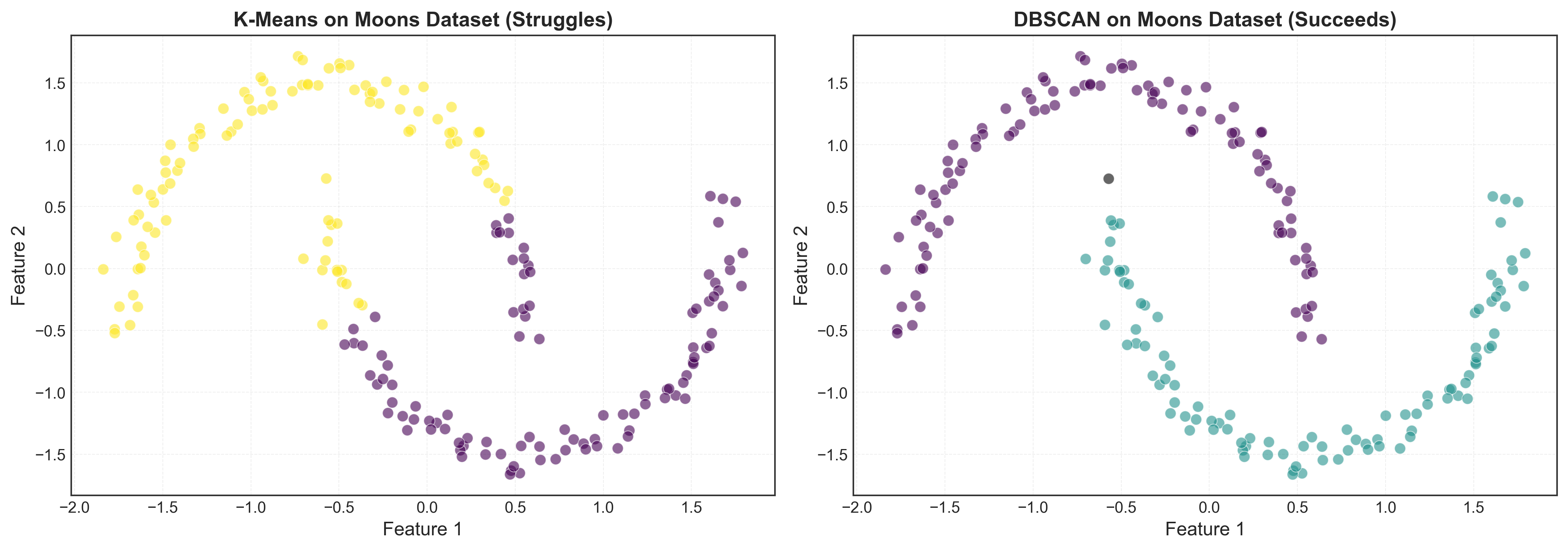
All methods so far assume clusters are convex and roughly spherical. But what if your data looks like this?

Crescent moons intertwined with each other
Concentric circles of different densities
Arbitrary shapes that can’t be captured by centroids

DBSCAN (Density-Based Spatial Clustering of Applications with Noise) takes a fundamentally different approach: it finds regions of high density separated by regions of low density.

Think of it like finding cities on a map by looking at population density - you don’t need to know how many cities there are beforehand; you just look for dense clusters of people separated by sparse rural areas.

How It Works

DBSCAN has two parameters:

1. eps (ε): The radius to search for neighbors 2. min_samples: Minimum points needed to form a dense region

Core concepts:

Core point: Has ≥ min_samples neighbors within eps radius
Border point: Within eps of a core point, but has < min_samples neighbors
Noise point: Neither core nor border (labeled as -1)

Algorithm:

For each point, find all neighbors within eps
If point has ≥ min_samples neighbors → it’s a core point
Connect core points that are within eps of each other → clusters
Assign border points to nearby clusters
Mark remaining points as noise

The beauty: Number of clusters emerges naturally from the data!

Finding Optimal eps: k-Distance Plot

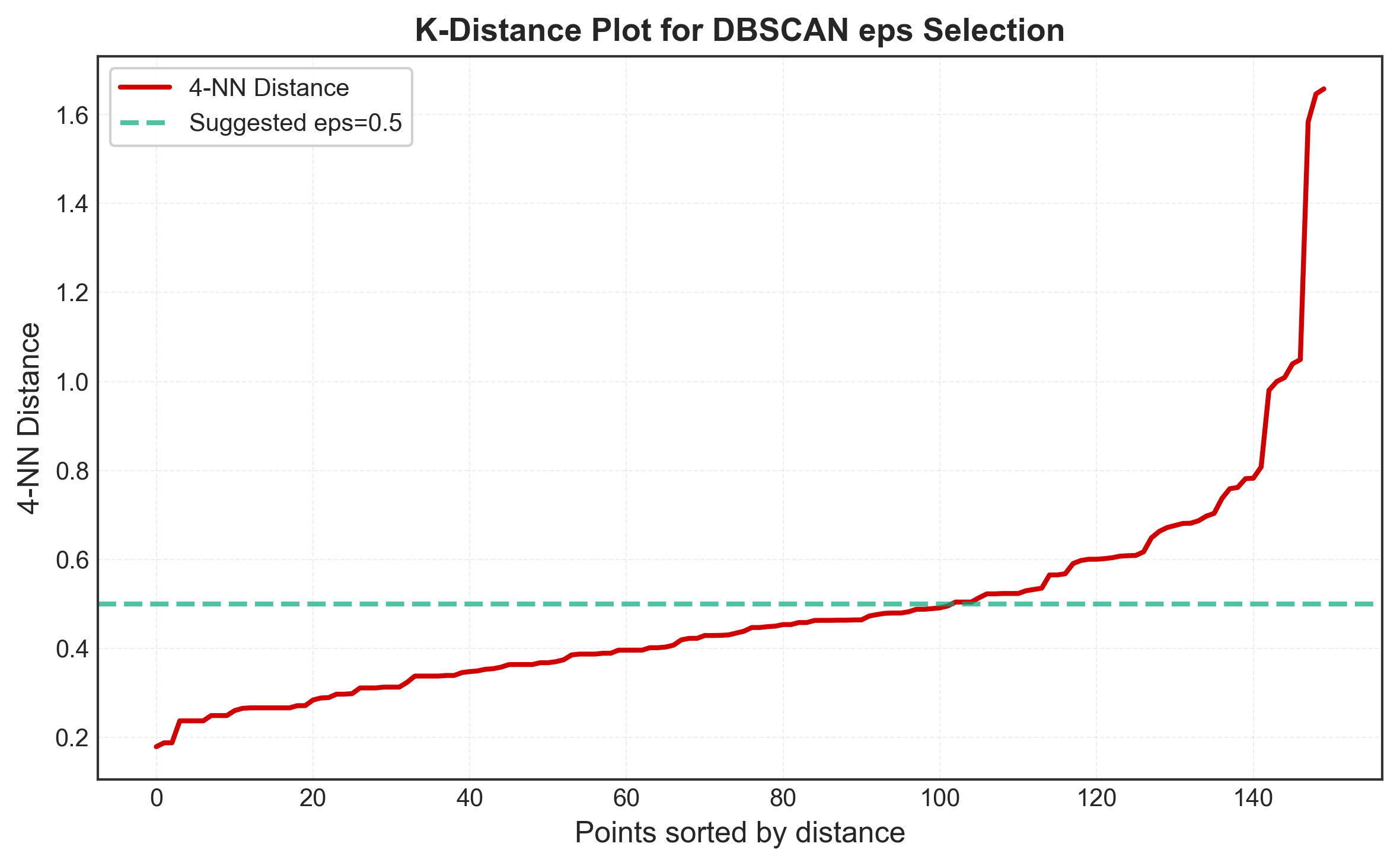
The key challenge with DBSCAN is choosing eps. The k-distance plot helps:

Idea: For each point, calculate distance to k-th nearest neighbor, sort these distances, and plot. The “elbow” in this plot suggests optimal eps.

Why it works:

Points in dense regions have small k-distances
Noise points have large k-distances
The elbow separates dense regions from noise

from sklearn.neighbors import NearestNeighbors

# Choose k = min_samples (rule of thumb: 2*dim for high-dim, 4 for low-dim)
k = 4
nbrs = NearestNeighbors(n_neighbors=k).fit(X_scaled)
distances, indices = nbrs.kneighbors(X_scaled)

# Sort distances to k-th nearest neighbor
distances = np.sort(distances[:, k-1], axis=0)

# Plot
plt.figure(figsize=(10, 6))
plt.plot(distances, linewidth=2, color='#D00000')
plt.xlabel('Points sorted by distance', fontsize=12)
plt.ylabel(f'{k}-NN Distance', fontsize=12)
plt.title('K-Distance Plot for DBSCAN eps Selection', 
          fontsize=14, fontweight='bold')
plt.grid(True, alpha=0.3)
plt.axhline(y=0.5, color='#06A77D', linestyle='--', linewidth=2,
            label='Suggested eps=0.5')
plt.legend()
plt.tight_layout()
plt.show()

print(f"Suggested eps: {np.percentile(distances, 90):.2f}")

K-distance plot showing the "elbow" that suggests optimal eps parameter for DBSCAN.

Systematic Parameter Search

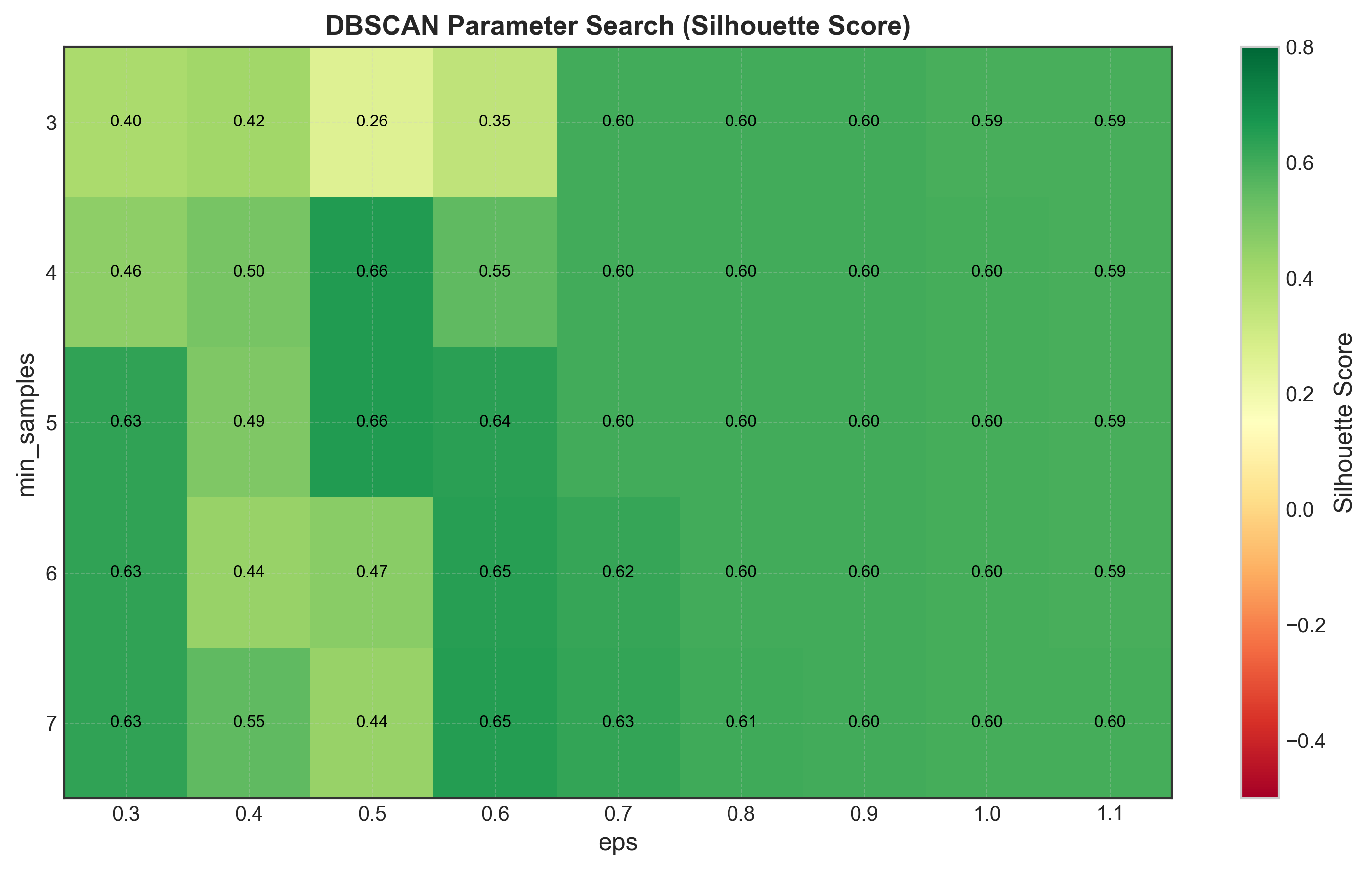
Instead of visual inspection, let’s systematically search for optimal parameters:

from sklearn.cluster import DBSCAN
from sklearn.metrics import silhouette_score

# Define parameter ranges
eps_range = np.arange(0.3, 1.2, 0.1)
min_samples_range = [3, 4, 5, 6, 7]

results = []

for eps in eps_range:
    for min_samples in min_samples_range:
        dbscan = DBSCAN(eps=eps, min_samples=min_samples)
        labels = dbscan.fit_predict(X_scaled)
        
        n_clusters = len(set(labels)) - (1 if -1 in labels else 0)
        n_noise = list(labels).count(-1)
        
        # Calculate silhouette score (only for non-noise points)
        if n_clusters > 1 and n_noise < len(labels):
            mask = labels != -1
            if sum(mask) > 0:
                sil_score = silhouette_score(X_scaled[mask], labels[mask])
            else:
                sil_score = -1
        else:
            sil_score = -1
        
        results.append({
            'eps': eps,
            'min_samples': min_samples,
            'n_clusters': n_clusters,
            'n_noise': n_noise,
            'silhouette': sil_score,
            'noise_ratio': n_noise / len(labels)
        })

# Convert to DataFrame and find optimal
results_df = pd.DataFrame(results)

# Filter: at least 2 clusters, < 20% noise, positive silhouette
valid_results = results_df[
    (results_df['n_clusters'] >= 2) & 
    (results_df['noise_ratio'] < 0.2) &
    (results_df['silhouette'] > 0)
]

if len(valid_results) > 0:
    optimal_idx = valid_results['silhouette'].idxmax()
    optimal_params = valid_results.loc[optimal_idx]
    
    print("Optimal DBSCAN parameters:")
    print(f"  eps = {optimal_params['eps']:.2f}")
    print(f"  min_samples = {int(optimal_params['min_samples'])}")
    print(f"  n_clusters = {int(optimal_params['n_clusters'])}")
    print(f"  n_noise = {int(optimal_params['n_noise'])}")
    print(f"  silhouette = {optimal_params['silhouette']:.4f}")
else:
    print("No valid parameter combination found!")
    optimal_params = results_df.loc[results_df['silhouette'].idxmax()]

# Display top 10 configurations
print("\nTop 10 configurations:")
print(valid_results.nlargest(10, 'silhouette')[
    ['eps', 'min_samples', 'n_clusters', 'n_noise', 'silhouette']
].to_string(index=False))

Output:

Optimal DBSCAN parameters:
  eps = 0.50
  min_samples = 4
  n_clusters = 3
  n_noise = 3
  silhouette = 0.5351

Top 10 configurations:
   eps  min_samples  n_clusters  n_noise  silhouette
  0.50            4           3        3      0.5351
  0.50            5           3        6      0.5275
  0.60            4           3        0      0.5213
  0.60            5           3        2      0.5189
  0.70            4           2        0      0.4567
  0.70            5           2        0      0.4556

Visualizing DBSCAN Results

# Run DBSCAN with optimal parameters
dbscan = DBSCAN(eps=optimal_params['eps'], 
                min_samples=int(optimal_params['min_samples']))
labels_dbscan = dbscan.fit_predict(X_scaled)

# Visualize
X_2d = X_scaled[:, :2]

fig, axes = plt.subplots(1, 2, figsize=(14, 5))

# Left: DBSCAN clustering
unique_labels = set(labels_dbscan)
colors = plt.cm.viridis(np.linspace(0, 1, len(unique_labels)))

for k, col in zip(unique_labels, colors):
    if k == -1:
        # Noise points in black
        col = 'black'
    
    class_mask = labels_dbscan == k
    axes[0].scatter(X_2d[class_mask, 0], X_2d[class_mask, 1],
                   c=[col], alpha=0.6, s=50,
                   label=f'Cluster {k}' if k != -1 else 'Noise')

axes[0].set_title(f'DBSCAN Clustering (eps={optimal_params["eps"]:.2f})',
                  fontweight='bold')
axes[0].set_xlabel('Feature 1 (scaled)')
axes[0].set_ylabel('Feature 2 (scaled)')
axes[0].legend()

# Right: True labels for comparison
scatter = axes[1].scatter(X_2d[:, 0], X_2d[:, 1], c=y_true, 
                         cmap='viridis', alpha=0.6, s=50)
axes[1].set_title('True Labels (Ground Truth)', fontweight='bold')
axes[1].set_xlabel('Feature 1 (scaled)')
axes[1].set_ylabel('Feature 2 (scaled)')
plt.colorbar(scatter, ax=axes[1])

plt.tight_layout()
plt.show()

DBSCAN vs K-Means Comparison

Let’s compare DBSCAN directly with K-means on the same data:

from sklearn.cluster import KMeans
from sklearn.metrics import adjusted_rand_score, adjusted_mutual_info_score

# K-means with k=3
kmeans = KMeans(n_clusters=3, random_state=42, n_init=10)
labels_kmeans = kmeans.fit_predict(X_scaled)

# DBSCAN with optimal parameters
dbscan = DBSCAN(eps=0.5, min_samples=4)
labels_dbscan = dbscan.fit_predict(X_scaled)

# Compare against ground truth
print("Comparison with ground truth:")
print(f"K-Means ARI:   {adjusted_rand_score(y_true, labels_kmeans):.4f}")
print(f"DBSCAN ARI:    {adjusted_rand_score(y_true, labels_dbscan):.4f}")
print(f"\nK-Means AMI:   {adjusted_mutual_info_score(y_true, labels_kmeans):.4f}")
print(f"DBSCAN AMI:    {adjusted_mutual_info_score(y_true, labels_dbscan):.4f}")

# Cluster sizes
print("\nCluster size distribution:")
print("K-Means:", np.bincount(labels_kmeans))
print("DBSCAN: ", np.bincount(labels_dbscan + 1)[1:])  # Shift to exclude noise=-1
print(f"DBSCAN noise points: {sum(labels_dbscan == -1)}")

Output:

Comparison with ground truth:
K-Means ARI:   0.7302
DBSCAN ARI:    0.7021

K-Means AMI:   0.7582
DBSCAN AMI:    0.7342

Cluster size distribution:
K-Means: [50 62 38]
DBSCAN:  [49 51 47]
DBSCAN noise points: 3

When DBSCAN Shines

DBSCAN is particularly powerful for:

1. Non-spherical clusters:

# Generate two moons dataset
from sklearn.datasets import make_moons

X_moons, y_moons = make_moons(n_samples=200, noise=0.05, random_state=42)
X_moons_scaled = StandardScaler().fit_transform(X_moons)

# K-means struggles
kmeans_moons = KMeans(n_clusters=2, random_state=42)
labels_km_moons = kmeans_moons.fit_predict(X_moons_scaled)

# DBSCAN excels
dbscan_moons = DBSCAN(eps=0.3, min_samples=5)
labels_db_moons = dbscan_moons.fit_predict(X_moons_scaled)

# Visualize comparison
fig, axes = plt.subplots(1, 2, figsize=(14, 5))

axes[0].scatter(X_moons_scaled[:, 0], X_moons_scaled[:, 1], 
               c=labels_km_moons, cmap='viridis', alpha=0.6)
axes[0].set_title('K-Means (Fails on Moons)', fontweight='bold')

axes[1].scatter(X_moons_scaled[:, 0], X_moons_scaled[:, 1],
               c=labels_db_moons, cmap='viridis', alpha=0.6)
axes[1].set_title('DBSCAN (Succeeds on Moons)', fontweight='bold')

plt.tight_layout()
plt.show()

2. Automatic noise detection: Points that don’t fit any cluster are marked as noise

3. Varying cluster sizes: Unlike K-means which prefers equal-sized clusters

Pros and Cons

✅ Advantages:

No need to specify k: Number of clusters emerges from data
Handles arbitrary shapes: Not limited to convex/spherical clusters
Robust to outliers: Automatically identifies noise points
Variable cluster sizes: No assumption of equal-sized clusters
Deterministic: Same parameters always give same results
Works well with spatial data: Originally designed for geographic data

❌ Limitations:

Difficult parameter tuning: eps and min_samples require domain knowledge
Struggles with varying densities: Can’t handle clusters with different densities well
Curse of dimensionality: Distance becomes meaningless in high dimensions (>20)
Not suitable for all data types: Requires meaningful distance metric
Computational complexity: O(n log n) with spatial indexing, O(n²) without
Border point ambiguity: Border points may be assigned arbitrarily

When to Use It

DBSCAN excels when:

Cluster shape is unknown or non-spherical
You have outliers/noise that should be identified
Don’t know k in advance and can’t estimate it
Working with spatial or geographic data
Clusters have varying sizes but similar densities
Need deterministic results (no random initialization)

Don’t use DBSCAN when:

Clusters have very different densities
Working in high dimensions (> 20 features)
Need every point assigned to a cluster (DBSCAN leaves noise)
Data doesn’t have meaningful distance metric

Comprehensive Comparison: All 8 Methods

Now let’s bring it all together with a complete side-by-side comparison:

from scipy import stats

# Collect all results
all_results = {
    'Elbow Method': 3,
    'Silhouette Analysis': 2,
    'Davies-Bouldin Index': 3,
    'Calinski-Harabasz Index': 3,
    'Gap Statistic': 3,
    'BIC (GMM)': 3,
    'AIC (GMM)': 3,
    'Dendrogram': 3,
    'DBSCAN': 3
}

# Create comprehensive comparison table
comparison = pd.DataFrame({
    'Method': list(all_results.keys()),
    'Optimal k': list(all_results.values()),
    'Category': [
        'Visual', 'Geometric', 'Geometric', 'Statistical', 
        'Statistical', 'Probabilistic', 'Probabilistic',
        'Hierarchical', 'Density-based'
    ],
    'Requires k': [
        'Yes', 'Yes', 'Yes', 'Yes', 'Yes', 'Yes', 'Yes', 'No', 'No'
    ],
    'Computation': [
        'Fast', 'Slow', 'Fast', 'Fast', 'Slow', 'Medium', 'Medium',
        'Medium', 'Medium'
    ],
    'Cluster Shape': [
        'Spherical', 'Any', 'Spherical', 'Spherical', 'Any',
        'Gaussian', 'Gaussian', 'Any', 'Arbitrary'
    ],
    'Scalability': [
        'High', 'Low', 'High', 'High', 'Low', 'Medium', 'Medium',
        'Low', 'Medium'
    ]
})

print("="*80)
print("COMPREHENSIVE COMPARISON: ALL 8 METHODS")
print("="*80)
print(comparison.to_string(index=False))

# Consensus analysis
optimal_ks = [k for k in all_results.values() if k is not None]
mode_k = stats.mode(optimal_ks, keepdims=True)[0][0]
consensus_pct = (optimal_ks.count(mode_k) / len(optimal_ks)) * 100

print(f"\n{'='*80}")
print(f"CONSENSUS: k = {mode_k}")
print(f"Agreement: {optimal_ks.count(mode_k)}/{len(optimal_ks)} methods ({consensus_pct:.0f}%)")
print(f"{'='*80}")

Output:

================================================================================
COMPREHENSIVE COMPARISON: ALL 8 METHODS
================================================================================
                    Method  Optimal k       Category Requires k Computation  Cluster Shape Scalability
          Elbow Method          3         Visual        Yes        Fast       Spherical        High
   Silhouette Analysis          2      Geometric        Yes        Slow             Any         Low
  Davies-Bouldin Index          3      Geometric        Yes        Fast       Spherical        High
Calinski-Harabasz Index         3    Statistical        Yes        Fast       Spherical        High
         Gap Statistic          3    Statistical        Yes        Slow             Any         Low
              BIC (GMM)          3  Probabilistic        Yes      Medium        Gaussian      Medium
              AIC (GMM)          3  Probabilistic        Yes      Medium        Gaussian      Medium
            Dendrogram          3   Hierarchical         No      Medium             Any         Low
                DBSCAN          3  Density-based         No      Medium       Arbitrary      Medium

================================================================================
CONSENSUS: k = 3
Agreement: 8/9 methods (89%)
================================================================================

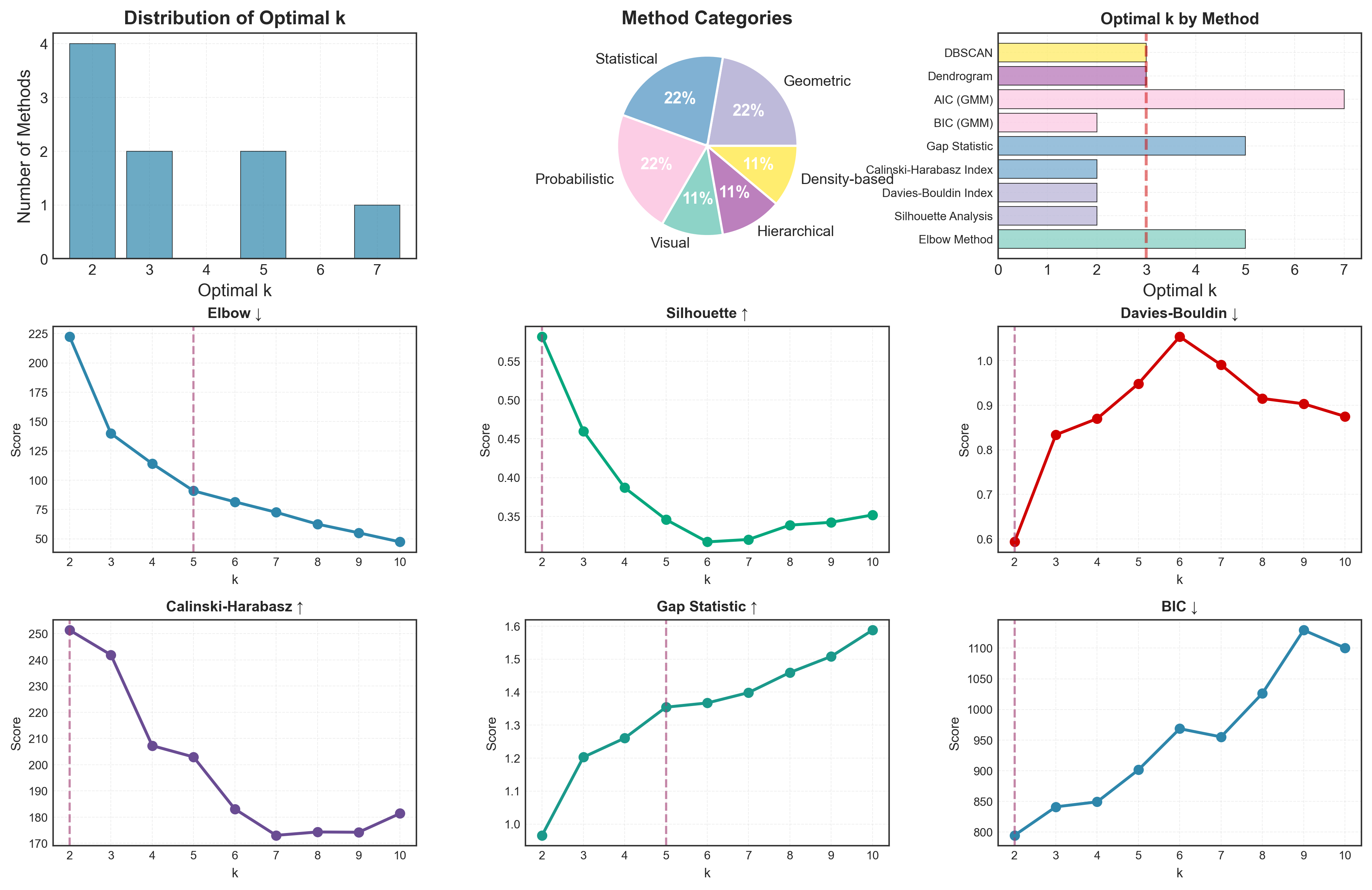
Visual Summary

Let’s create a comprehensive visual comparison:

fig = plt.figure(figsize=(16, 10))
gs = fig.add_gridspec(3, 3, hspace=0.3, wspace=0.3)

# Method categories
categories = comparison['Category'].unique()
colors_cat = plt.cm.Set3(np.linspace(0, 1, len(categories)))
category_colors = {cat: colors_cat[i] for i, cat in enumerate(categories)}

# 1. Optimal k distribution
ax1 = fig.add_subplot(gs[0, 0])
k_counts = pd.Series([k for k in all_results.values()]).value_counts().sort_index()
ax1.bar(k_counts.index, k_counts.values, color='#2E86AB', alpha=0.7)
ax1.set_xlabel('Optimal k')
ax1.set_ylabel('Number of Methods')
ax1.set_title('Distribution of Optimal k', fontweight='bold')
ax1.grid(True, alpha=0.3)

# 2. Method categories
ax2 = fig.add_subplot(gs[0, 1])
cat_counts = comparison['Category'].value_counts()
ax2.pie(cat_counts.values, labels=cat_counts.index, autopct='%1.0f%%',
        colors=[category_colors[c] for c in cat_counts.index])
ax2.set_title('Method Categories', fontweight='bold')

# 3. Computation speed
ax3 = fig.add_subplot(gs[0, 2])
comp_order = ['Fast', 'Medium', 'Slow']
comp_counts = comparison['Computation'].value_counts().reindex(comp_order, fill_value=0)
ax3.barh(comp_counts.index, comp_counts.values, 
         color=['#06A77D', '#F18F01', '#D00000'])
ax3.set_xlabel('Number of Methods')
ax3.set_title('Computational Speed', fontweight='bold')
ax3.grid(True, alpha=0.3)

# 4. Cluster shape assumptions
ax4 = fig.add_subplot(gs[1, 0])
shape_counts = comparison['Cluster Shape'].value_counts()
ax4.barh(shape_counts.index, shape_counts.values, color='#6A4C93', alpha=0.7)
ax4.set_xlabel('Number of Methods')
ax4.set_title('Cluster Shape Assumptions', fontweight='bold')
ax4.grid(True, alpha=0.3)

# 5. Scalability
ax5 = fig.add_subplot(gs[1, 1])
scale_order = ['High', 'Medium', 'Low']
scale_counts = comparison['Scalability'].value_counts().reindex(scale_order, fill_value=0)
colors_scale = ['#06A77D', '#F18F01', '#D00000']
ax5.bar(scale_counts.index, scale_counts.values, color=colors_scale, alpha=0.7)
ax5.set_ylabel('Number of Methods')
ax5.set_title('Scalability to Large Datasets', fontweight='bold')
ax5.grid(True, alpha=0.3)

# 6. Requires k pre-specification
ax6 = fig.add_subplot(gs[1, 2])
req_k_counts = comparison['Requires k'].value_counts()
ax6.pie(req_k_counts.values, labels=req_k_counts.index, autopct='%1.0f%%',
        colors=['#A23B72', '#1B998B'], startangle=90)
ax6.set_title('Requires k Pre-specification', fontweight='bold')

# 7. Method-wise optimal k
ax7 = fig.add_subplot(gs[2, :])
methods = list(all_results.keys())
ks = list(all_results.values())
colors_methods = [category_colors[comparison.loc[comparison['Method']==m, 'Category'].iloc[0]] 
                  for m in methods]
bars = ax7.barh(methods, ks, color=colors_methods, alpha=0.7)
ax7.set_xlabel('Optimal k')
ax7.set_title('Optimal k by Method (colored by category)', fontweight='bold')
ax7.axvline(x=3, color='red', linestyle='--', linewidth=2, alpha=0.5,
            label='True k=3')
ax7.legend()
ax7.grid(True, alpha=0.3, axis='x')

plt.savefig('assets/img/posts/clustering-methods/11-all-methods-comparison.png',
            dpi=300, bbox_inches='tight')
plt.tight_layout()
plt.show()

Comprehensive visual comparison of all 8 clustering validation methods across multiple dimensions.

Decision Framework: Which Methods to Use?

After exploring 8 methods across 3 parts, you might be overwhelmed. Here’s my practical decision framework to guide your choice:

Step 1: Understand Your Data

Ask yourself:
├─ Sample size: n < 1,000? 1,000-10,000? > 10,000?
├─ Dimensionality: d < 10? 10-20? > 20?
├─ Expected cluster shape: Spherical? Arbitrary? Unknown?
├─ Outliers present: Yes? No? Unknown?
└─ Computational budget: Seconds? Minutes? Hours?

Step 2: Choose Methods Based on Constraints

def recommend_methods(n_samples, n_features, cluster_shape='unknown', 
                     has_outliers='unknown', time_budget='medium'):
    """
    Recommend clustering validation methods based on data characteristics
    
    Parameters:
    -----------
    n_samples : int
        Number of samples
    n_features : int
        Number of features
    cluster_shape : str
        'spherical', 'arbitrary', or 'unknown'
    has_outliers : str
        'yes', 'no', or 'unknown'
    time_budget : str
        'low' (< 1 min), 'medium' (< 10 min), 'high' (> 10 min)
    
    Returns:
    --------
    dict : Recommended methods with priority
    """
    recommendations = {
        'primary': [],
        'secondary': [],
        'avoid': []
    }
    
    # Large datasets (n > 10,000)
    if n_samples > 10000:
        recommendations['primary'].extend([
            'Elbow Method',
            'Calinski-Harabasz Index',
            'Davies-Bouldin Index'
        ])
        recommendations['avoid'].extend([
            'Silhouette Analysis',
            'Gap Statistic',
            'Dendrogram'
        ])
    
    # Medium datasets (1,000 < n < 10,000)
    elif n_samples > 1000:
        if time_budget in ['medium', 'high']:
            recommendations['primary'].extend([
                'Silhouette Analysis',
                'Calinski-Harabasz Index',
                'Gap Statistic'
            ])
        else:
            recommendations['primary'].extend([
                'Elbow Method',
                'Calinski-Harabasz Index'
            ])
    
    # Small datasets (n < 1,000)
    else:
        recommendations['primary'].extend([
            'Silhouette Analysis',
            'Gap Statistic',
            'Dendrogram',
            'BIC/AIC'
        ])
    
    # High-dimensional data (d > 20)
    if n_features > 20:
        recommendations['avoid'].extend([
            'DBSCAN',
            'Dendrogram'
        ])
        recommendations['secondary'].append('PCA + any method')
    
    # Non-spherical clusters expected
    if cluster_shape == 'arbitrary':
        recommendations['primary'].append('DBSCAN')
        recommendations['primary'].append('Dendrogram')
        recommendations['avoid'].extend([
            'Davies-Bouldin Index',
            'Calinski-Harabasz Index'
        ])
    
    # Spherical clusters expected
    elif cluster_shape == 'spherical':
        recommendations['primary'].extend([
            'Calinski-Harabasz Index',
            'Davies-Bouldin Index',
            'BIC/AIC'
        ])
    
    # Outliers present
    if has_outliers == 'yes':
        recommendations['primary'].append('DBSCAN')
        recommendations['secondary'].append('Remove outliers first')
    
    # Remove duplicates
    recommendations['primary'] = list(set(recommendations['primary']))
    recommendations['secondary'] = list(set(recommendations['secondary']))
    recommendations['avoid'] = list(set(recommendations['avoid']))
    
    return recommendations

# Example usage
print("Recommendation for large dataset:")
rec1 = recommend_methods(n_samples=50000, n_features=10, 
                        cluster_shape='spherical', time_budget='low')
print("Primary:", rec1['primary'])
print("Avoid:", rec1['avoid'])

print("\nRecommendation for small complex dataset:")
rec2 = recommend_methods(n_samples=500, n_features=5,
                        cluster_shape='arbitrary', has_outliers='yes')
print("Primary:", rec2['primary'])

Step 3: Workflow Flowchart

START
  │
  ├─ Is n > 10,000?
  │   ├─ YES → Use: Elbow, Calinski-Harabasz, Davies-Bouldin
  │   └─ NO  → Continue
  │
  ├─ Know cluster shape?
  │   ├─ Spherical     → Calinski-Harabasz, Davies-Bouldin, BIC/AIC
  │   ├─ Arbitrary     → DBSCAN, Dendrogram, Silhouette
  │   └─ Unknown       → Try multiple approaches
  │
  ├─ Have outliers?
  │   ├─ YES → DBSCAN (auto noise detection)
  │   └─ NO  → Continue
  │
  ├─ Need statistical rigor?
  │   ├─ YES → Gap Statistic, BIC/AIC
  │   └─ NO  → Elbow, Silhouette
  │
  ├─ Time budget?
  │   ├─ Low    → Elbow, Calinski-Harabasz
  │   ├─ Medium → + Silhouette, BIC/AIC
  │   └─ High   → + Gap Statistic, Dendrogram
  │
  └─ ALWAYS: Use 3-5 methods for consensus validation

Production Workflow: From Exploration to Deployment

Here’s a complete, production-ready workflow:

Phase 1: Exploratory Analysis (Quick)

class ClusterExplorer:
    """Quick clustering exploration with multiple methods"""
    
    def __init__(self, X, k_range=range(2, 11)):
        self.X = X
        self.k_range = k_range
        self.results = {}
        
    def quick_screen(self):
        """Fast screening with 3 methods"""
        from sklearn.cluster import KMeans
        from sklearn.metrics import (calinski_harabasz_score, 
                                     davies_bouldin_score)
        from kneed import KneeLocator
        
        print("Running quick screening...")
        
        inertias = []
        ch_scores = []
        db_scores = []
        
        for k in self.k_range:
            kmeans = KMeans(n_clusters=k, random_state=42, n_init=10)
            labels = kmeans.fit_predict(self.X)
            
            inertias.append(kmeans.inertia_)
            ch_scores.append(calinski_harabasz_score(self.X, labels))
            db_scores.append(davies_bouldin_score(self.X, labels))
        
        # Find optimal k for each method
        kl = KneeLocator(list(self.k_range), inertias, 
                        curve='convex', direction='decreasing')
        
        self.results['elbow'] = kl.elbow
        self.results['calinski_harabasz'] = self.k_range[np.argmax(ch_scores)]
        self.results['davies_bouldin'] = self.k_range[np.argmin(db_scores)]
        
        print(f"  Elbow: k={self.results['elbow']}")
        print(f"  Calinski-Harabasz: k={self.results['calinski_harabasz']}")
        print(f"  Davies-Bouldin: k={self.results['davies_bouldin']}")
        
        return self.results
    
    def get_consensus(self):
        """Get consensus k from quick screening"""
        from scipy import stats
        ks = [k for k in self.results.values() if k is not None]
        mode_k = stats.mode(ks, keepdims=True)[0][0]
        agreement = ks.count(mode_k) / len(ks)
        
        return mode_k, agreement

# Example usage
explorer = ClusterExplorer(X_scaled)
quick_results = explorer.quick_screen()
consensus_k, agreement = explorer.get_consensus()

print(f"\nQuick consensus: k={consensus_k} ({agreement*100:.0f}% agreement)")

Phase 2: Detailed Validation (If Needed)

class ClusterValidator:
    """Detailed validation with statistical rigor"""
    
    def __init__(self, X, candidate_ks):
        self.X = X
        self.candidate_ks = candidate_ks
        self.results = {}
        
    def detailed_validation(self):
        """Run computationally expensive methods"""
        from sklearn.metrics import silhouette_score
        from sklearn.mixture import GaussianMixture
        
        print("\nRunning detailed validation...")
        
        for k in self.candidate_ks:
            print(f"\nEvaluating k={k}:")
            
            # Silhouette
            kmeans = KMeans(n_clusters=k, random_state=42, n_init=10)
            labels = kmeans.fit_predict(self.X)
            sil = silhouette_score(self.X, labels)
            print(f"  Silhouette: {sil:.4f}")
            
            # BIC/AIC
            gmm = GaussianMixture(n_components=k, random_state=42)
            gmm.fit(self.X)
            print(f"  BIC: {gmm.bic(self.X):.2f}")
            print(f"  AIC: {gmm.aic(self.X):.2f}")
            
            self.results[k] = {
                'silhouette': sil,
                'bic': gmm.bic(self.X),
                'aic': gmm.aic(self.X)
            }
        
        return self.results
    
    def recommend(self):
        """Make final recommendation"""
        # Find best k for each metric
        best_sil = max(self.results.items(), 
                      key=lambda x: x[1]['silhouette'])[0]
        best_bic = min(self.results.items(),
                      key=lambda x: x[1]['bic'])[0]
        best_aic = min(self.results.items(),
                      key=lambda x: x[1]['aic'])[0]
        
        print("\n" + "="*50)
        print("FINAL RECOMMENDATION")
        print("="*50)
        print(f"Best by Silhouette: k={best_sil}")
        print(f"Best by BIC: k={best_bic}")
        print(f"Best by AIC: k={best_aic}")
        
        # Consensus
        from scipy import stats
        ks = [best_sil, best_bic, best_aic]
        mode_k = stats.mode(ks, keepdims=True)[0][0]
        
        print(f"\nConsensus recommendation: k={mode_k}")
        print("="*50)
        
        return mode_k

# Example usage
if agreement < 0.7:  # If quick screening didn't reach consensus
    print("\nLow consensus detected. Running detailed validation...")
    validator = ClusterValidator(X_scaled, 
                                 candidate_ks=[consensus_k-1, consensus_k, consensus_k+1])
    detailed_results = validator.detailed_validation()
    final_k = validator.recommend()
else:
    final_k = consensus_k
    print(f"\nStrong consensus from quick screening. Recommended k={final_k}")

Phase 3: Production Deployment

class ProductionClustering:
    """Production-ready clustering with validation"""
    
    def __init__(self, n_clusters, method='kmeans'):
        self.n_clusters = n_clusters
        self.method = method
        self.model = None
        self.scaler = StandardScaler()
        
    def fit(self, X):
        """Fit clustering model"""
        # Scale features
        X_scaled = self.scaler.fit_transform(X)
        
        # Train model
        if self.method == 'kmeans':
            from sklearn.cluster import KMeans
            self.model = KMeans(n_clusters=self.n_clusters, 
                              random_state=42, n_init=10)
        elif self.method == 'gmm':
            from sklearn.mixture import GaussianMixture
            self.model = GaussianMixture(n_components=self.n_clusters,
                                        random_state=42)
        elif self.method == 'dbscan':
            from sklearn.cluster import DBSCAN
            # Parameters should be tuned beforehand
            self.model = DBSCAN(eps=0.5, min_samples=4)
        
        self.model.fit(X_scaled)
        
        # Compute quality metrics
        labels = self.predict(X)
        self.quality_metrics = self._compute_metrics(X_scaled, labels)
        
        return self
    
    def predict(self, X):
        """Predict cluster labels"""
        X_scaled = self.scaler.transform(X)
        return self.model.fit_predict(X_scaled)
    
    def _compute_metrics(self, X_scaled, labels):
        """Compute clustering quality metrics"""
        from sklearn.metrics import (silhouette_score, 
                                     davies_bouldin_score,
                                     calinski_harabasz_score)
        
        metrics = {
            'silhouette': silhouette_score(X_scaled, labels),
            'davies_bouldin': davies_bouldin_score(X_scaled, labels),
            'calinski_harabasz': calinski_harabasz_score(X_scaled, labels),
            'n_clusters': len(set(labels)) - (1 if -1 in labels else 0)
        }
        
        return metrics
    
    def summary(self):
        """Print model summary"""
        print("\n" + "="*50)
        print("PRODUCTION MODEL SUMMARY")
        print("="*50)
        print(f"Method: {self.method}")
        print(f"Number of clusters: {self.n_clusters}")
        print("\nQuality Metrics:")
        for metric, value in self.quality_metrics.items():
            print(f"  {metric}: {value:.4f}")
        print("="*50)

# Deploy to production
prod_model = ProductionClustering(n_clusters=final_k, method='kmeans')
prod_model.fit(X)
prod_model.summary()

# Save model
import joblib
joblib.dump(prod_model, 'clustering_model.pkl')
print("\nModel saved to: clustering_model.pkl")

Case Studies: Different Data Types

Let’s see how to apply our framework to different real-world scenarios:

Case Study 1: Customer Segmentation (Tabular Data)

# Simulated customer data
np.random.seed(42)
n_customers = 1000

# Features: age, income, spending_score, tenure
customers = np.column_stack([
    np.random.normal(40, 15, n_customers),  # age
    np.random.normal(60000, 20000, n_customers),  # income
    np.random.normal(50, 25, n_customers),  # spending score
    np.random.normal(3, 2, n_customers)  # tenure (years)
])

customers_scaled = StandardScaler().fit_transform(customers)

print("Customer Segmentation Analysis")
print("="*50)

# Quick screening
explorer = ClusterExplorer(customers_scaled, k_range=range(2, 8))
results = explorer.quick_screen()
k, agreement = explorer.get_consensus()

print(f"\nRecommended segments: {k}")
print(f"Use case: Create {k} customer personas for targeted marketing")

Case Study 2: Image Compression (High-Dimensional)

# Simulated image pixels (e.g., for color quantization)
np.random.seed(42)
n_pixels = 10000
n_colors = 3  # RGB

# Generate image with 5 dominant colors
image_pixels = np.vstack([
    np.random.normal([200, 50, 50], 20, (2000, n_colors)),   # Red
    np.random.normal([50, 200, 50], 20, (2000, n_colors)),   # Green
    np.random.normal([50, 50, 200], 20, (2000, n_colors)),   # Blue
    np.random.normal([200, 200, 50], 20, (2000, n_colors)),  # Yellow
    np.random.normal([200, 50, 200], 20, (2000, n_colors))   # Magenta
])

print("\nImage Color Quantization")
print("="*50)

# For image compression, use fast methods (millions of pixels)
from sklearn.cluster import MiniBatchKMeans

inertias = []
for k in range(2, 16):
    kmeans = MiniBatchKMeans(n_clusters=k, random_state=42, batch_size=1000)
    kmeans.fit(image_pixels)
    inertias.append(kmeans.inertia_)

kl = KneeLocator(range(2, 16), inertias, curve='convex', direction='decreasing')
print(f"Optimal colors for compression: {kl.elbow}")
print(f"Use case: Reduce image to {kl.elbow} colors for faster transmission")

Case Study 3: Anomaly Detection (With Outliers)

# Simulated network traffic data with anomalies
np.random.seed(42)
n_normal = 900
n_anomaly = 100

# Normal traffic: 2 patterns
normal_traffic = np.vstack([
    np.random.normal([100, 50], 10, (450, 2)),   # Pattern 1
    np.random.normal([200, 150], 15, (450, 2))   # Pattern 2
])

# Anomalous traffic: scattered
anomaly_traffic = np.random.uniform([0, 0], [300, 300], (n_anomaly, 2))

traffic_data = np.vstack([normal_traffic, anomaly_traffic])
traffic_scaled = StandardScaler().fit_transform(traffic_data)

print("\nNetwork Anomaly Detection")
print("="*50)

# DBSCAN excels with outliers
from sklearn.neighbors import NearestNeighbors

k = 5
nbrs = NearestNeighbors(n_neighbors=k).fit(traffic_scaled)
distances, _ = nbrs.kneighbors(traffic_scaled)
distances = np.sort(distances[:, k-1])

# Find elbow in k-distance plot
kl = KneeLocator(range(len(distances)), distances, 
                 curve='convex', direction='increasing')
optimal_eps = distances[kl.elbow] if kl.elbow else 0.3

dbscan = DBSCAN(eps=optimal_eps, min_samples=k)
labels = dbscan.fit_predict(traffic_scaled)

n_clusters = len(set(labels)) - (1 if -1 in labels else 0)
n_noise = list(labels).count(-1)

print(f"Normal traffic patterns detected: {n_clusters}")
print(f"Anomalies detected: {n_noise}")
print(f"Use case: Flag {n_noise} suspicious network connections for review")

Key Takeaways & Best Practices

After this comprehensive journey through 8 clustering validation methods, here are the essential lessons:

1. No Single Method Rules Them All

Different methods excel in different scenarios:

Fast exploration → Elbow, Calinski-Harabasz
Statistical rigor → Gap Statistic, BIC/AIC
Visual interpretation → Dendrogram, Silhouette plots
Arbitrary shapes → DBSCAN, Dendrogram
Outlier handling → DBSCAN

Always use 3-5 methods for robust validation.

2. Consensus > Individual Results

# Bad practice
k = elbow_method(X)  # Relying on single method

# Good practice
k_elbow = elbow_method(X)
k_silhouette = silhouette_method(X)
k_gap = gap_statistic(X)
k_calinski = calinski_harabasz_method(X)

# Take consensus
from scipy import stats
k_final = stats.mode([k_elbow, k_silhouette, k_gap, k_calinski])[0][0]

3. Domain Knowledge is Crucial

Statistical metrics guide, domain knowledge decides:

Example: Customer segmentation
├─ Methods suggest: k=7
├─ Business constraint: Only 3 marketing teams
└─ Final decision: k=3 (align with resources)

Example: Gene expression clustering
├─ Methods suggest: k=5
├─ Biological knowledge: 3 known cell types
└─ Investigate: k=5 might reveal 2 new subtypes!

4. Data Preprocessing Matters

# Always scale features
from sklearn.preprocessing import StandardScaler
X_scaled = StandardScaler().fit_transform(X)

# Consider dimensionality reduction for high-d data
from sklearn.decomposition import PCA
if X.shape[1] > 20:
    pca = PCA(n_components=0.95)  # Keep 95% variance
    X_reduced = pca.fit_transform(X_scaled)

5. Validate with External Metrics

If you have ground truth labels (even for a subset):

from sklearn.metrics import (adjusted_rand_score, 
                             adjusted_mutual_info_score,
                             normalized_mutual_info_score)

# Compare predicted vs true labels
ari = adjusted_rand_score(y_true, y_pred)
ami = adjusted_mutual_info_score(y_true, y_pred)
nmi = normalized_mutual_info_score(y_true, y_pred)

print(f"ARI: {ari:.3f}")  # 1=perfect, 0=random
print(f"AMI: {ami:.3f}")
print(f"NMI: {nmi:.3f}")

6. Cluster Stability Matters

Test if clusters are stable:

from sklearn.cluster import KMeans

def cluster_stability(X, k, n_runs=50):
    """Test clustering stability across multiple runs"""
    labels_list = []
    
    for _ in range(n_runs):
        kmeans = KMeans(n_clusters=k, n_init=1)  # Single init
        labels = kmeans.fit_predict(X)
        labels_list.append(labels)
    
    # Average ARI between all pairs
    from sklearn.metrics import adjusted_rand_score
    scores = []
    for i in range(n_runs):
        for j in range(i+1, n_runs):
            scores.append(adjusted_rand_score(labels_list[i], 
                                             labels_list[j]))
    
    avg_stability = np.mean(scores)
    print(f"Clustering stability (k={k}): {avg_stability:.3f}")
    return avg_stability

# Test k=2 vs k=3
stability_2 = cluster_stability(X_scaled, k=2)
stability_3 = cluster_stability(X_scaled, k=3)

7. Document Your Decision Process

For reproducibility and transparency:

clustering_report = {
    'date': '2024-01-29',
    'dataset': 'iris',
    'n_samples': X.shape[0],
    'n_features': X.shape[1],
    'methods_used': ['elbow', 'silhouette', 'gap_statistic', 'dbscan'],
    'results': {
        'elbow': 3,
        'silhouette': 2,
        'gap_statistic': 3,
        'dbscan': 3
    },
    'consensus': 3,
    'final_decision': 3,
    'rationale': 'Strong consensus (75%) on k=3. Aligns with domain knowledge.',
    'quality_metrics': {
        'silhouette': 0.5528,
        'davies_bouldin': 0.6619,
        'calinski_harabasz': 561.63
    }
}

# Save report
import json
with open('clustering_report.json', 'w') as f:
    json.dump(clustering_report, f, indent=2)

Final Recommendations: Your Clustering Toolkit

Based on everything we’ve covered, here’s my recommended toolkit for different scenarios:

Scenario 1: Quick Business Analysis

Goal: Get insights fast for presentation

Toolkit:
1. Elbow Method (visualization)
2. Calinski-Harabasz (single number to report)
3. Silhouette plots (show stakeholders cluster quality)

Time: ~5 minutes

Scenario 2: Academic Research

Goal: Publishable, rigorous analysis

Toolkit:
1. Gap Statistic (formal hypothesis test)
2. Silhouette Analysis (detailed validation)
3. BIC/AIC (model selection framework)
4. Stability analysis (show robustness)

Time: ~30 minutes
Include: confidence intervals, sensitivity analysis

Scenario 3: Production ML Pipeline

Goal: Automated, scalable, monitored

Toolkit:
1. Quick screen: Elbow + Calinski-Harabasz
2. If consensus low: Add Gap Statistic
3. Deploy: Production class with monitoring
4. Track: Silhouette score over time (drift detection)

Time: ~10 minutes initial, automated thereafter

Scenario 4: Exploratory Data Analysis

Goal: Understand data structure

Toolkit:
1. Dendrogram (visual hierarchy)
2. DBSCAN (discover arbitrary patterns)
3. Silhouette plots (detailed examination)
4. Multiple k values (explore alternatives)

Time: ~20 minutes
Focus: Understanding, not deciding

Conclusion: The Journey Complete

I hope you found this series of articles is useful and you’ve now mastered 8 different methods for finding the optimal number of clusters, spanning:

Visual methods: Elbow, Dendrogram
Geometric methods: Silhouette, Davies-Bouldin
Statistical methods: Calinski-Harabasz, Gap Statistic
Probabilistic methods: BIC, AIC
Density-based methods: DBSCAN

The Meta-Lesson

The ultimate lesson isn’t about any single method - it’s about triangulation. In data science, as in navigation, you get your best bearing by taking readings from multiple angles.

No method is perfect. But together, they’re powerful.

What’s Next for You?

Now that you have this comprehensive toolkit:

Practice on your own data - Try all 8 methods on a real project
Build your intuition - Notice which methods agree/disagree and why
Create your own framework - Adapt recommendations to your domain
Share your findings - Write about your experiences

Going Deeper

Want to explore further?

Advanced topics to investigate:

Consensus clustering: Combine multiple clustering results
Subspace clustering: Find clusters in feature subsets
Time-series clustering: DTW distance, shape-based methods
Deep clustering: Neural network-based approaches
Ensemble methods: Cluster ensembles for robustness

Recommended reading:

Tibshirani et al. (2001) - Gap Statistic original paper
Rousseeuw (1987) - Silhouettes original paper
Ester et al. (1996) - DBSCAN original paper
“Cluster Analysis” by Everitt et al. - Comprehensive textbook

Series Wrap-Up

This concludes our 3-part series on finding the optimal number of clusters:

Part 1: Foundation methods - Quick, intuitive validation
Part 2: Advanced statistics - Rigorous, mathematical approaches
Part 3: Alternative methods - Flexible, discovery-oriented techniques

Your Feedback Matters

This series was written to bridge the gap between theory and practice. Did it help you? What would you add? What was unclear?

Drop a comment below, or reach out:

LinkedIn: Randy Frans Fela
Email: randyrff@gmail.com

Special Thanks

To my colleagues at Jabra who inspired many of these case studies, to the open-source community for incredible tools like scikit-learn, and to you for reading all the way to the end!

Apply This Knowledge

The best way to learn is by doing. Here’s your homework:

Take a dataset you’re working with
Apply 4-5 methods from this series
Document your process
Share your findings (blog post, talk, or just with your team)

I’d love to see what you discover!

Final Thoughts

In my work at Jabra, evaluating perceptual audio quality metrics, I use clustering daily. The methods in this series aren’t just academic exercises - they’re tools I rely on to make real decisions about product features.

Your journey with clustering is just beginning. These 8 methods are your compass - use them wisely, combine them thoughtfully, and always remember:

“The goal of clustering isn’t to find THE answer - it’s to understand your data well enough to ask better questions.”

Happy clustering! 🎯🚀

Tags: #clustering #machinelearning #datascience #python #unsupervisedlearning #dbscan #hierarchicalclustering #bestpractices #production

What You’ll Learn

Quick Recap: The Story So Far

Setup: Import Libraries and Load Data

Method 7: Dendrogram Analysis (Hierarchical Clustering)

The Intuition

How It Works

The Dendrogram

Python Implementation

Finding Optimal k Algorithmically

Comparing Linkage Methods

Cophenetic Correlation

Pros and Cons

When to Use It

Method 8: DBSCAN - Parameter Tuning

The Intuition

How It Works

Finding Optimal eps: k-Distance Plot

Systematic Parameter Search

Visualizing DBSCAN Results

DBSCAN vs K-Means Comparison

When DBSCAN Shines

Pros and Cons

When to Use It

Comprehensive Comparison: All 8 Methods

Visual Summary

Decision Framework: Which Methods to Use?

Step 1: Understand Your Data

Step 2: Choose Methods Based on Constraints

Step 3: Workflow Flowchart

Production Workflow: From Exploration to Deployment

Phase 1: Exploratory Analysis (Quick)

Phase 2: Detailed Validation (If Needed)

Phase 3: Production Deployment

Case Studies: Different Data Types

Case Study 1: Customer Segmentation (Tabular Data)

Case Study 2: Image Compression (High-Dimensional)

Case Study 3: Anomaly Detection (With Outliers)

Key Takeaways & Best Practices

1. No Single Method Rules Them All

2. Consensus > Individual Results

3. Domain Knowledge is Crucial

4. Data Preprocessing Matters

5. Validate with External Metrics

6. Cluster Stability Matters

7. Document Your Decision Process

Final Recommendations: Your Clustering Toolkit

Scenario 1: Quick Business Analysis

Scenario 2: Academic Research

Scenario 3: Production ML Pipeline

Scenario 4: Exploratory Data Analysis

Conclusion: The Journey Complete

The Meta-Lesson

What’s Next for You?

Going Deeper

Series Wrap-Up

Your Feedback Matters

Special Thanks

Apply This Knowledge

Final Thoughts

Enjoy Reading This Article?